How Query Engines Think: The Tradeoffs Behind Every Data System

Read the complete Query Engine Optimization series:

Part 1: How Query Engines Think: The Tradeoffs Behind Every Data System
Part 2: Row vs. Column: How Storage Layout Shapes Everything
Part 3: How Databases Organize Data on Disk: Pages, Blocks, and File Formats
Part 4: B-Trees, LSM Trees, and the Indexing Tradeoff Spectrum
Part 5: Inside the Query Optimizer: How Engines Pick a Plan
Part 6: Volcano, Vectorized, Compiled: How Engines Execute Your Query
Part 7: Buffer Pools, Caches, and the Memory Hierarchy
Part 8: Partitioning, Sharding, and Data Distribution Strategies
Part 9: Hash, Sort-Merge, Broadcast: How Distributed Joins Work
Part 10: Concurrency, Isolation, and MVCC: How Engines Handle Contention Every database you have ever used is a collection of deliberate engineering tradeoffs. PostgreSQL is fast at looking up a single customer record but slow at scanning a billion rows for an aggregate. ClickHouse is the opposite. DuckDB runs analytical queries on your laptop at speeds that embarrass some cloud data warehouses, but it is not designed to handle 10,000 concurrent transactional writes per second. Dremio accelerates analytical queries on lakehouse data using Apache Arrow and Iceberg, but it is not a replacement for a transactional OLTP database.

None of these systems are broken. They are each optimized for a specific set of problems, and that optimization comes at the cost of other problems. Understanding why they behave differently requires looking at the nine design decisions that every query engine must make.

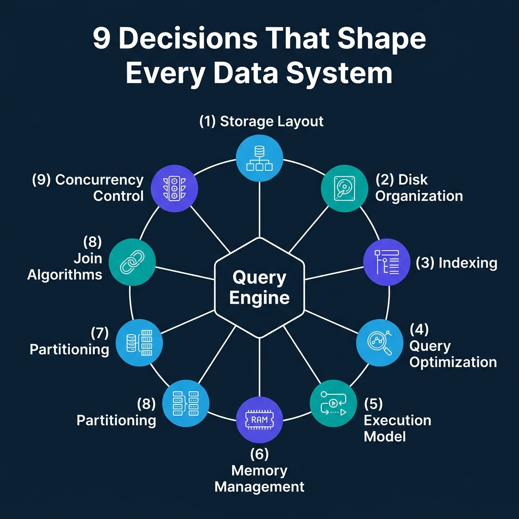
The 9 decisions that shape every query engine from storage layout to concurrency control

The Nine Decisions Every Engine Must Make

When engineers build a query engine, they face a series of interconnected choices. Each choice optimizes for one type of workload and creates a weakness for another. Here is the full map:

Storage layout: Should records be stored by row or by column?
Disk organization: How should data be structured within files? What metadata should accompany it?
Indexing: What auxiliary data structures should speed up lookups?
Query optimization: How should the engine choose between multiple possible execution strategies?
Execution model: How should the CPU actually process data through the operator tree?
Memory management: How should the engine use RAM, and what happens when data does not fit?
Partitioning: How should data be divided across storage units or nodes?
Join algorithms: When data for a join lives in different places, how do you bring it together?
Concurrency control: How should the engine handle multiple transactions touching the same data?

The rest of this article introduces each area. The nine articles that follow will cover each one in depth.

Storage Layout: Row vs. Column

The most fundamental decision is how to arrange bytes on disk.

Row stores (PostgreSQL, MySQL) keep all fields of a record physically adjacent. When you look up a customer by ID, the engine reads one contiguous block and has every field immediately. Inserts and updates are fast because the entire record lives in one place.

Column stores (DuckDB, ClickHouse, Dremio, Snowflake) keep all values for a single field stored together. When an analytical query needs the average of one column across a billion rows, the engine reads only that column and ignores the other 49. Compression improves because uniform data types pack tightly. But inserting a single row means writing to every column file separately.

Dimension	Row Store	Column Store
Point lookups	Fast (one read gets full record)	Slow (must read from every column)
Analytical scans	Slow (reads unused columns)	Fast (reads only needed columns)
Compression	Moderate (mixed types)	High (uniform types, 5-10x better)
Transactional writes	Fast (one write per record)	Expensive (one write per column)

The choice cascades through everything else: what indexes make sense, how execution works, how memory is used. It is the first domino.

How Data Gets Indexed

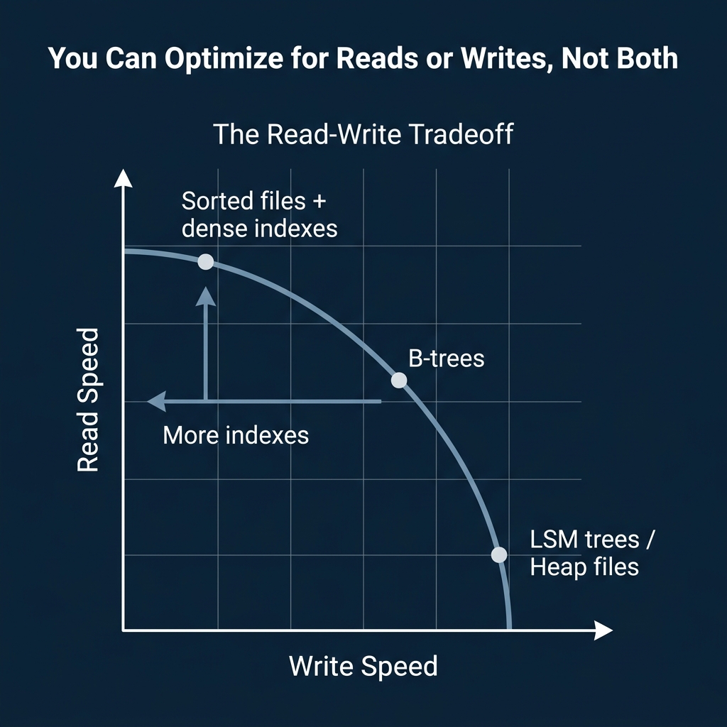
Every index speeds up reads and slows down writes. The question is which tradeoff to accept.

B-trees are the standard for transactional databases. They maintain a balanced tree structure with O(log n) lookups and efficient range scans. PostgreSQL, MySQL, and Oracle all default to B-trees. They handle mixed read/write workloads well, but heavy write volumes cause fragmentation and rebalancing overhead.

LSM trees (Log-Structured Merge-Trees) are built for write-heavy workloads. They buffer writes in memory and flush them to disk as sorted files, converting random writes into sequential ones. RocksDB, Cassandra, and HBase all use LSM trees. The tradeoff: reads may need to check multiple levels of sorted files before finding the answer.

Zone maps and min/max indexes are the columnar engine’s answer. Store the minimum and maximum value for each data block. When a query filters on that column, skip every block whose range does not overlap the filter. No write overhead, but only useful for scan-heavy workloads.

The read-write tradeoff showing how sorted files with dense indexes optimize reads while LSM trees and heap files optimize writes

Planning and Executing the Query

Once data is stored and indexed, the engine must decide how to answer your query.

Query optimizers choose between candidate execution plans. A rule-based optimizer applies fixed transformations (push filters down, drop unused columns). A cost-based optimizer estimates the cost of multiple plans using table statistics and picks the cheapest one. Spark’s Adaptive Query Execution goes further: it monitors actual data sizes during execution and changes the plan mid-flight.

The tradeoff: more planning time can find dramatically better plans, but the planning itself has a cost. For a simple point lookup, an elaborate cost-based search is wasted effort. For a complex 12-table join, skipping cost-based optimization can produce a plan that is 100x slower than necessary.

Execution models determine how the CPU processes data through the plan:

Volcano (iterator): Each operator passes one row at a time via Next() calls. Simple, modular, but millions of virtual function calls waste CPU cycles on large datasets. PostgreSQL uses this model.
Vectorized: Each Next() call returns a batch of rows (e.g., 1024). Tight inner loops process one column at a time, exploiting CPU SIMD instructions. DuckDB, ClickHouse, and Dremio use this approach.
Code generation: Fuse multiple operators into a single compiled function. Eliminate operator abstraction entirely. Apache Spark’s Tungsten engine uses whole-stage code generation.

Memory, Distribution, and Concurrency

The remaining decisions shape how the engine handles scale and contention.

Memory management is a balancing act. More RAM for caching means faster repeated reads. More RAM for sort buffers and hash tables means faster query processing. The engine cannot maximize both. Traditional databases use buffer pools that pin frequently accessed pages in memory. Analytical engines use column-level caches and result caches.

Partitioning determines how data is divided. Hash partitioning distributes data evenly but makes range scans expensive. Range partitioning makes range scans fast but creates hotspots when keys are skewed. The optimizer’s ability to skip irrelevant partitions (partition pruning) is often the single biggest performance win in large-scale systems.

Join algorithms in distributed systems face a fundamental problem: data for a join may live on different nodes. A shuffle join re-distributes both tables by the join key across the network. A broadcast join copies the small table to every node. A co-located join requires that both tables were pre-partitioned by the same key, avoiding data movement entirely.

Concurrency control decides what happens when multiple transactions touch the same data. Two-phase locking (2PL) is safe but limits throughput because readers block writers. MVCC (Multi-Version Concurrency Control) keeps multiple row versions so readers see a consistent snapshot without blocking writers. Most modern systems, from PostgreSQL to Dremio and Snowflake, use MVCC or snapshot-based isolation.

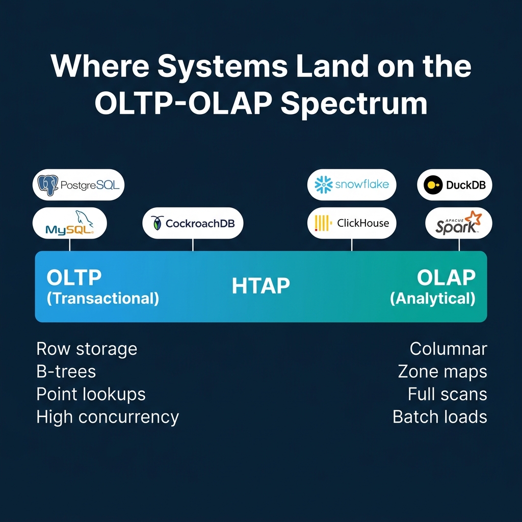
The OLTP-OLAP Spectrum

All nine decisions converge on one fundamental axis: is this system built for transactions or analytics?

Where real-world database systems land on the OLTP to OLAP design spectrum

Dimension	OLTP Optimization	OLAP Optimization
Storage	Row-oriented	Column-oriented
Indexing	B-trees	Zone maps, bloom filters
Access pattern	Point lookups, small updates	Full scans, aggregations
Execution	Volcano (row-at-a-time)	Vectorized / compiled
Concurrency	High (MVCC, fine-grained locks)	Low (batch loads, snapshots)
Distribution	Sharding by primary key	MPP with shuffle joins

No single system dominates both ends. Systems that attempt Hybrid Transactional/Analytical Processing (HTAP) make explicit compromises, typically maintaining two internal storage formats and routing queries to whichever is more appropriate.

Where This Series Goes Next

This overview is the map. The nine articles that follow are the territory:

Row vs. Column Storage: how physical byte layout determines which queries are fast
Data Organization on Disk: pages, blocks, file formats, and metadata
Indexing Strategies: B-trees, LSM trees, bitmap indexes, and bloom filters
Query Optimizer Internals: cost-based planning, cardinality estimation, and adaptive execution
Execution Models: Volcano, vectorized, compiled, and morsel-driven parallelism
Memory Management and Caching: buffer pools, cache eviction, and spill strategies
Partitioning and Data Distribution: hash, range, bucketing, and partition pruning
Distributed Join Algorithms: shuffle, broadcast, co-located, and the cost of data movement
Concurrency and Isolation: locks, MVCC, isolation levels, and optimistic concurrency

Each article covers one decision area with diagrams, real-world system examples, and the specific tradeoffs involved. The goal is not to pick winners but to understand how the engineers who build these systems think through the problems.